SeekOps’ dynamic uncertainty method sets a new standard for methane measurement accuracy by analyzing in situ variables like wind, temperature, and pressure, and dynamically propagating uncertainty to deliver transparent, defensible emissions data.
Read time: 5 minutes
When it comes to measuring methane emissions, knowing how much is only part of the story. Equally important is understanding how confident we can be in that number.
At SeekOps, our technology doesn’t just detect and quantify methane, it also quantifies the uncertainty in every measurement, based on the actual real time survey conditions. This framework, which we call dynamic uncertainty, brings transparency, traceability, and scientific rigor to methane emissions data.
Why Uncertainty Estimation Matters
In environmental monitoring, uncertainty is not a weakness; it’s an acknowledgment of reality. Every emission quantification is influenced by multiple variables: sensor precision, wind speed and direction, temperature gradients, atmospheric turbulence, and model assumptions.
Many methane measurement systems handle this complexity by assigning a fixed uncertainty across all measurements. But the real atmosphere doesn’t behave that way. Each survey has its own meteorology, each plume its own structure, and each flight its own sampling geometry.
At SeekOps, we believe every emission requires its own uncertainty assessment, one that reflects what actually happened in the field. That’s the foundation of dynamic uncertainty.
From Components to Confidence: The Physics of the Flux Plane
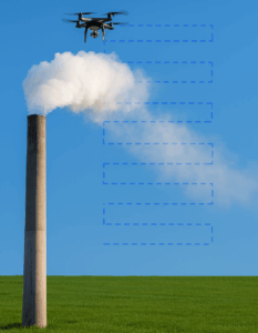
Our quantification framework begins with the flux plane, the core output of SeekOps’ methane quantification system. The flux plane represents a vertical, gridded slice of the atmosphere that captures methane concentration enhancements along the drone’s flight path.
Each grid cell corresponds to an integrated measurement of methane mixing ratio, air density (measured by temperature and pressure), and wind speed. When combined, these data reconstruct a 2D flux field which is essentially a picture of how methane moves through the air at a given moment.
Mathematically, the total mass flux through the plane is computed as:
$$
\dot{m}_i = \frac{M_i}{M_{\text{air}}}
\sum_{y,z} \rho_{\text{air}}(y,z) \,
\chi_i(y,z) \,
u_{\perp}(y,z) \,
\Delta y \, \Delta z
\tag{1}
$$
Where:
• ρair: dry air density (from in situ pressure & temperature)
• χi: measured methane enhancement mole fraction
• u⊥: wind velocity component normal to the plane
• Mi/Mair: molar mass ratio of methane to dry air
• Δy, Δz : grid spacing in the horizontal and vertical directions, respectively
The integration of all these cells yields the total methane emission rate for the surveyed source (ṁi). Note that wind direction factors in here as u⊥ = u cos(Φ) where Φ is the angle between the incident wind direction and the flux plane normal vector.
Step 1: Decomposing the Sources of Error
The first step in quantifying dynamic uncertainty is identifying where uncertainty comes from. Some of these sources were described by Mohammadloo et al. (2025) and include:
• Instrument errors — from the SeekIR methane sensor and onboard environmental sensors (relatively small contributor).
• Environmental variability — fluctuating winds, turbulence, and thermal stratification (moderate contributor).
• Sampling geometry — how well the drone’s flight pattern intersects the plume (largest contributor).
• Model assumptions — simplifications made in the mass balance and atmospheric transport equations.
At SeekOps, our emission solution explicitly measures the variables that influence some of these error sources. So, we can put it all together to see how each contributes to the overall uncertainty in our delivered emission rate.
Step 2: Defining the Error Propagation Framework
The flux plane’s uncertainty is computed using optimal estimation theory, a framework originally developed for satellite and lidar retrievals (e.g., Rodgers, 2000; Burton et al., 2016).
We define the measurement state vector as:
$$
\textbf{x} \in
\begin{cases}
\Delta \textrm{y} &: \text{distance along the flux plane},\\
\Delta \textrm{z} &: \text{vertical step of drone intervals},\\
u &: \text{wind speed},\\
\theta &: \text{wind direction},\\
T &: \text{temperature},\\
P &: \text{pressure},\\
\chi &: \text{gas enhancement concentration}
\end{cases}
$$
and the forward model F(x) that outputs the retrieved mass flux is given by Eq. (1).
Uncertainty is then propagated by differentiating the mass balance equation per each state parameter using central finite differencing which applies first-order Taylor expansion to ignore high order terms. This process builds the Jacobian matrix (K).
Covariance matrices that describe the empirical variability from controlled release studies (presented in Corbett and Smith, 2022), instrument accuracy, and measurement variability are constructed and propagated with K per the optimal estimation framework.
The terms in our error propagation framework are:
| Term | Symbol | Description |
| Jacobian Matrix | K | Partial derivatives of the forward model with respect to each state variable. This helps quantify sensitivity to errors in individual state measurements. |
| Random Error Covariance Matrix | Sr | Representing sensor noise and background signal variance |
| Empirical Error | Se | Controlled releases from Corbett and Smith (2022) show a 1 sigma accuracy of ± 30%. This is accounted for here. |
| State Vector Covariance | Sm | Represents the correlation between measured state variables |
| Spatial Grid Covariance | Sg | Represents the correlation among pixels on the flux plane grid. Here is where any large changes in environmental conditions across the grid are captured. |
Step 3: Building the Covariance Matrices
The total prior covariance matrix combines random, measurement, and empirical components:
$$
S_\textrm{a}=S_\textrm{r}+S_\textrm{m}+S_\textrm{e}
$$
Each term plays a specific role:
• Sr: random measurement noise
• Sm: atmospheric state variable correlations
• Se: empirical uncertainty (~30% derived from validation campaigns)
The posterior covariance matrix incorporates correlation across the flux plane grid and state variable sensitivity through the Jacobian:
$$
S_\textrm{p}=\left( K^TS_\textrm{g}^{-1}K+S_\textrm{a}^{-1}\right)^{-1}
$$
Here, K represents the forward model sensitivity matrix (Jacobian) and Sg is the measurement covariance across the flux plane grid.
These matrices allow SeekOps to translate the field measurements into gridded uncertainty estimates and state variable uncertainty components, showing not only how much methane was detected but also how reliable each part of the plane is, and which state variables contribute most to the overall error.
Step 4: Visualizing the Uncertainty Grid
Once the covariance and Jacobian are computed, the uncertainty is reshaped into a 2D spatial grid corresponding to the flux plane geometry.
Each grid cell now contains a local estimate of uncertainty (σ) in the same units as the mass flux (e.g., kg/hr). The uncertainty grid looks similar to our plume concentration enhancements as the highest uncertainty typically occurs in the same spatial region where the signal is strongest, because that is where the model is doing the most “work.” In contrast, areas far outside the plume contribute almost nothing to the mass flux calculation, so even if there is noise there, its impact on the final emission estimate is negligible. As a result, the uncertainty naturally concentrates where the plume energy is, reflecting where errors actually matter.
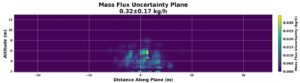
- The top image shows the spatial distribution of uncertainty. Brighter areas indicate regions of greater variability — for instance, where the plume edges were only partially captured or where wind shear increased error propagation.
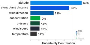
- The bottom chart visualizes a state parameter sensitivity analysis, showing how much each variable (wind, concentration, temperature, etc.) contributes to the total uncertainty.
- Together, these visualizations demonstrate how dynamic uncertainty converts complex retrieval theory into an intuitive map of measurement confidence.
Finally, the total uncertainty is computed as the quadrature sum of the gridded variances:
$$
\sigma_{\textrm{total}}=\sqrt{\sum_{\textrm{i}}\sigma_{\textrm{i}}^2}
$$
and reported as a one-standard-deviation range on the emission estimate:
$$
M_{\textrm{i}}\pm\sigma_{\textrm{total}}
$$
Step 5: Interpreting Dynamic Uncertainty in the Field
Dynamic uncertainty means that every SeekOps emission rate reflects its true field context.
• In steady, well-defined plume conditions, uncertainty tightens.
• In variable atmospheres and ill-defined plume geometries, it widens.
Rather than masking that variability, we make it visible. Each measurement’s confidence is quantified and mapped, providing operators and regulators with a transparent view of what’s known, and what’s less certain.
This empowers operators to:
• Compare sites and surveys with statistical rigor.
• Prioritize mitigation based on both emission size and confidence.
• Defend results in ESG or regulatory reporting with traceable mathematical justification.
Looking Ahead: Beyond Dynamic Uncertainty
Dynamic uncertainty is the first half of a broader quantification philosophy. The next stage of SeekOps’ framework will address scenario uncertainty: accounting for “what if” cases like plumes drifting between flight lines or unmeasured variability in time.
Together, these two frameworks will deliver a total uncertainty envelope, encompassing both measurable and inferential confidence limits, an industry first for drone-based methane quantification.
How Uncertainty Transparency Informs the Future Standard
By making uncertainty visible, quantified, and tied directly to real field conditions, SeekOps is enabling the industry to move beyond “black box” emissions reporting and toward evidence-based methane accountability. This level of transparency is exactly what emerging regulatory frameworks, methane intensity certifications, and voluntary reporting programs are beginning to demand, not just a number, but how confident we are in that number.
As methane standards evolve, the expectation will shift from simply reporting emissions to demonstrating defensibility, being able to show why a measurement should be trusted, how it responds to weather and operational conditions, and how it compares across time and technologies. SeekOps’ dynamic uncertainty framework future-proofs operators by aligning directly with this direction of travel. It transforms methane quantification from a static output into a traceable, decision-grade dataset, the foundation required for what will become the next generation of international measurement standards.
References
Corbett, A., & Smith, B. (2022). Study of a Miniature TDLAS System Onboard Two Unmanned Aircraft to Independently Quantify Methane Emissions from Oil and Gas Production Assets and Other Industrial Emitters. Atmosphere, 13(5), 804. https://doi.org/10.3390/atmos13050804
Burton, S. P., Hair, J. W., et. al. (2016). Observations of the spectral dependence of linear particle depolarization ratio of aerosols using NASA Langley airborne High Spectral Resolution Lidar. Atmospheric Measurement Techniques, 9, 5555–5572. https://doi.org/10.5194/amt-9-5555-2016
Rodgers, C. D. (2000). Inverse Methods for Atmospheric Sounding: Theory and Practice. World Scientific.